AutoEncoder自动编码器
Deep Learning最简单的一种方法是利用人工神经网络的特点,人工神经网络(ANN)本身就是具有层次结构的系统,如果给定一个神经网络,我们假设其输出与输入是相同的,然后训练调整其参数,得到每一层中的权重。自然地,我们就得到了输入I的几种不同表示(每一层代表一种表示),这些表示就是特征。自动编码器就是一种尽可能复现输入信号的神经网络。为了实现这种复现,自动编码器就必须捕捉可以代表输入数据的最重要的因素,就像PCA那样,找到可以代表原信息的主要成分。
具体过程简单的说明如下:
1)给定无标签数据,用非监督学习学习特征:

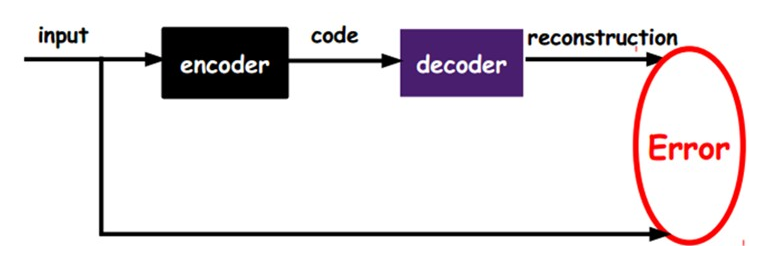
在我们之前的神经网络中,如第一个图,我们输入的样本是有标签的,即(input, target),这样我们根据当前输出和target(label)之间的差去改变前面各层的参数,直到收敛。但现在我们只有无标签数据,也就是右边的图。那么这个误差怎么得到呢?

如上图,我们将input输入一个encoder编码器,就会得到一个code,这个code也就是输入的一个表示,那么我们怎么知道这个code表示的就是input呢?我们加一个decoder解码器,这时候decoder就会输出一个信息,那么如果输出的这个信息和一开始的输入信号input是很像的(理想情况下就是一样的),那很明显,我们就有理由相信这个code是靠谱的。所以,我们就通过调整encoder和decoder的参数,使得重构误差最小,这时候我们就得到了输入input信号的第一个表示了,也就是编码code了。因为是无标签数据,所以误差的来源就是直接重构后与原输入相比得到。

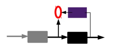
2)通过编码器产生特征,然后训练下一层。这样逐层训练:
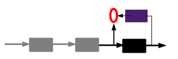
那上面我们就得到第一层的code,我们的重构误差最小让我们相信这个code就是原输入信号的良好表达了,或者牵强点说,它和原信号是一模一样的(表达不一样,反映的是一个东西)。那第二层和第一层的训练方式就没有差别了,我们将第一层输出的code当成第二层的输入信号,同样最小化重构误差,就会得到第二层的参数,并且得到第二层输入的code,也就是原输入信息的第二个表达了。其他层就同样的方法炮制就行了(训练这一层,前面层的参数都是固定的,并且他们的decoder已经没用了,都不需要了)。

3)有监督微调:
经过上面的方法,我们就可以得到很多层了。至于需要多少层(或者深度需要多少,这个目前本身就没有一个科学的评价方法)需要自己试验调了。每一层都会得到原始输入的不同的表达。当然了,我们觉得它是越抽象越好了,就像人的视觉系统一样。
到这里,这个AutoEncoder还不能用来分类数据,因为它还没有学习如何去连结一个输入和一个类。它只是学会了如何去重构或者复现它的输入而已。或者说,它只是学习获得了一个可以良好代表输入的特征,这个特征可以最大程度上代表原输入信号。那么,为了实现分类,我们就可以在AutoEncoder的最顶的编码层添加一个分类器(例如罗杰斯特回归、SVM等),然后通过标准的多层神经网络的监督训练方法(梯度下降法)去训练。
也就是说,这时候,我们需要将最后层的特征code输入到最后的分类器,通过有标签样本,通过监督学习进行微调,这也分两种,一个是只调整分类器(黑色部分):

另一种:通过有标签样本,微调整个系统:(如果有足够多的数据,这个是最好的。end-to-end learning端对端学习)

一旦监督训练完成,这个网络就可以用来分类了。神经网络的最顶层可以作为一个线性分类器,然后我们可以用一个更好性能的分类器去取代它。
在研究中可以发现,如果在原有的特征中加入这些自动学习得到的特征可以大大提高精确度,甚至在分类问题中比目前最好的分类算法效果还要好!
An autoencoder takes an inputand first maps it (with an_encoder)_to a hidden representationthrough a deterministic mapping, e.g.:
Where s is a non-linearity such as the sigmoid. The latent representation y , or code is then mapped back (with a_decoder)_into a reconstruction z of the same shape as x. The mapping happens through a similar transformation, e.g.:
(Here, the prime symbol does not indicate matrix transposition.) z should be seen as a prediction of x , given the code y . Optionally, the weight matrix of the reverse mapping may be constrained to be the transpose of the forward mapping: This is referred to astied weights. The parameters of this model (namely W, b , and, if one doesn’t use tied weights, also ) are optimized such that the average reconstruction error is minimized.
The reconstruction error can be measured in many ways, depending on the appropriate distributional assumptions on the input given the code. The traditionalsquared error, can be used. If the input is interpreted as either bit vectors or vectors of bit probabilities,_cross-entropy_of the reconstruction can be used:
The hope is that the code y is adistributed_representation that captures the coordinates along the main factors of variation in the data. This is similar to the way the projection on principal components would capture the main factors of variation in the data. Indeed, if there is one linear hidden layer (the_code)_and the mean squared error criterion is used to train the network, then the k hidden units learn to project the input in the span of the first k principal components of the data. If the hidden layer is non-linear, the auto-encoder behaves differently from PCA, with the ability to capture multi-modal aspects of the input distribution. The departure from PCA becomes even more important when we consider_stacking multiple encoders(and their corresponding decoders) when building a deep auto-encoder[Hinton06].
Because y is viewed as a lossy compression of x, it cannot be a good (small-loss) compression for all x. Optimization makes it a good compression for training examples, and hopefully for other inputs as well, but not for arbitrary inputs. That is the sense in which an auto-encoder generalizes: it gives low reconstruction error on test examples from the same distribution as the training examples, but generally high reconstruction error on samples randomly chosen from the input space.
We want to implement an auto-encoder using Theano, in the form of a class, that could be afterwards used in constructing a stacked autoencoder. The first step is to create shared variables for the parameters of the autoencoder W, b and . (Since we are using tied weights in this tutorial,will be used for ):
    def __init__(
        self,
        numpy_rng,
        theano_rng=None,
        input=None,
        n_visible=784,
        n_hidden=500,
        W=None,
        bhid=None,
        bvis=None
    ):
        """
        Initialize the dA class by specifying the number of visible units (the
        dimension d of the input ), the number of hidden units ( the dimension
        d' of the latent or hidden space ) and the corruption level. The
        constructor also receives symbolic variables for the input, weights and
        bias. Such a symbolic variables are useful when, for example the input
        is the result of some computations, or when weights are shared between
        the dA and an MLP layer. When dealing with SdAs this always happens,
        the dA on layer 2 gets as input the output of the dA on layer 1,
        and the weights of the dA are used in the second stage of training
        to construct an MLP.

        :type numpy_rng: numpy.random.RandomState
        :param numpy_rng: number random generator used to generate weights

        :type theano_rng: theano.tensor.shared_randomstreams.RandomStreams
        :param theano_rng: Theano random generator; if None is given one is
                     generated based on a seed drawn from `rng`

        :type input: theano.tensor.TensorType
        :param input: a symbolic description of the input or None for
                      standalone dA

        :type n_visible: int
        :param n_visible: number of visible units

        :type n_hidden: int
        :param n_hidden:  number of hidden units

        :type W: theano.tensor.TensorType
        :param W: Theano variable pointing to a set of weights that should be
                  shared belong the dA and another architecture; if dA should
                  be standalone set this to None

        :type bhid: theano.tensor.TensorType
        :param bhid: Theano variable pointing to a set of biases values (for
                     hidden units) that should be shared belong dA and another
                     architecture; if dA should be standalone set this to None

        :type bvis: theano.tensor.TensorType
        :param bvis: Theano variable pointing to a set of biases values (for
                     visible units) that should be shared belong dA and another
                     architecture; if dA should be standalone set this to None


        """
        self.n_visible = n_visible
        self.n_hidden = n_hidden

        # create a Theano random generator that gives symbolic random values
        if not theano_rng:
            theano_rng = RandomStreams(numpy_rng.randint(2 ** 30))

        # note : W' was written as `W_prime` and b' as `b_prime`
        if not W:
            # W is initialized with `initial_W` which is uniformely sampled
            # from -4*sqrt(6./(n_visible+n_hidden)) and
            # 4*sqrt(6./(n_hidden+n_visible))the output of uniform if
            # converted using asarray to dtype
            # theano.config.floatX so that the code is runable on GPU
            initial_W = numpy.asarray(
                numpy_rng.uniform(
                    low=-4 * numpy.sqrt(6. / (n_hidden + n_visible)),
                    high=4 * numpy.sqrt(6. / (n_hidden + n_visible)),
                    size=(n_visible, n_hidden)
                ),
                dtype=theano.config.floatX
            )
            W = theano.shared(value=initial_W, name='W', borrow=True)

        if not bvis:
            bvis = theano.shared(
                value=numpy.zeros(
                    n_visible,
                    dtype=theano.config.floatX
                ),
                borrow=True
            )

        if not bhid:
            bhid = theano.shared(
                value=numpy.zeros(
                    n_hidden,
                    dtype=theano.config.floatX
                ),
                name='b',
                borrow=True
            )

        self.W = W
        # b corresponds to the bias of the hidden
        self.b = bhid
        # b_prime corresponds to the bias of the visible
        self.b_prime = bvis
        # tied weights, therefore W_prime is W transpose
        self.W_prime = self.W.T
        self.theano_rng = theano_rng
        # if no input is given, generate a variable representing the input
        if input is None:
            # we use a matrix because we expect a minibatch of several
            # examples, each example being a row
            self.x = T.dmatrix(name='input')
        else:
            self.x = input

        self.params = [self.W, self.b, self.b_prime]
Note that we pass the symbolicinputto the autoencoder as a parameter. This is so that we can concatenate layers of autoencoders to form a deep network: the symbolic output (the y above) of layer k will be the symbolic input of layer k+1
Now we can express the computation of the latent representation and of the reconstructed signal:
def get_hidden_values(self, input):
    """ Computes the values of the hidden layer """
    return T.nnet.sigmoid(T.dot(input, self.W) + self.b)
def get_reconstructed_input(self, hidden):
    """Computes the reconstructed input given the values of the
    hidden layer
    """
    return T.nnet.sigmoid(T.dot(hidden, self.W_prime) + self.b_prime)
And using these functions we can compute the cost and the updates of one stochastic gradient descent step:
    def get_cost_updates(self, corruption_level, learning_rate):
        """ This function computes the cost and the updates for one trainng
        step of the dA """

        tilde_x = self.get_corrupted_input(self.x, corruption_level)
        y = self.get_hidden_values(tilde_x)
        z = self.get_reconstructed_input(y)
        # note : we sum over the size of a datapoint; if we are using
        #        minibatches, L will be a vector, with one entry per
        #        example in minibatch
        L = - T.sum(self.x * T.log(z) + (1 - self.x) * T.log(1 - z), axis=1)
        # note : L is now a vector, where each element is the
        #        cross-entropy cost of the reconstruction of the
        #        corresponding example of the minibatch. We need to
        #        compute the average of all these to get the cost of
        #        the minibatch
        cost = T.mean(L)

        # compute the gradients of the cost of the `dA` with respect
        # to its parameters
        gparams = T.grad(cost, self.params)
        # generate the list of updates
        updates = [
            (param, param - learning_rate * gparam)
            for param, gparam in zip(self.params, gparams)
        ]

        return (cost, updates)
We can now define a function that applied iteratively will update the parametersW,bandb_primesuch that the reconstruction cost is approximately minimized.
    da = dA(
        numpy_rng=rng,
        theano_rng=theano_rng,
        input=x,
        n_visible=28 * 28,
        n_hidden=500
    )

    cost, updates = da.get_cost_updates(
        corruption_level=0.,
        learning_rate=learning_rate
    )

    train_da = theano.function(
        [index],
        cost,
        updates=updates,
        givens={
            x: train_set_x[index * batch_size: (index + 1) * batch_size]
        }
    )

    start_time = timeit.default_timer()

    ############
    # TRAINING #
    ############

    # go through training epochs
    for epoch in range(training_epochs):
        # go through trainng set
        c = []
        for batch_index in range(n_train_batches):
            c.append(train_da(batch_index))

        print('Training epoch %d, cost ' % epoch, numpy.mean(c, dtype='float64'))

    end_time = timeit.default_timer()

    training_time = (end_time - start_time)

    print(('The no corruption code for file ' +
           os.path.split(__file__)[1] +
           ' ran for %.2fm' % ((training_time) / 60.)), file=sys.stderr)
    image = Image.fromarray(
        tile_raster_images(X=da.W.get_value(borrow=True).T,
                           img_shape=(28, 28), tile_shape=(10, 10),
                           tile_spacing=(1, 1)))
    image.save('filters_corruption_0.png')

    # start-snippet-3
    #####################################
    # BUILDING THE MODEL CORRUPTION 30% #
    #####################################

    rng = numpy.random.RandomState(123)
    theano_rng = RandomStreams(rng.randint(2 ** 30))

    da = dA(
        numpy_rng=rng,
        theano_rng=theano_rng,
        input=x,
        n_visible=28 * 28,
        n_hidden=500
    )

    cost, updates = da.get_cost_updates(
        corruption_level=0.3,
        learning_rate=learning_rate
    )

    train_da = theano.function(
        [index],
        cost,
        updates=updates,
        givens={
            x: train_set_x[index * batch_size: (index + 1) * batch_size]
        }
    )

    start_time = timeit.default_timer()

    ############
    # TRAINING #
    ############

    # go through training epochs
    for epoch in range(training_epochs):
        # go through trainng set
        c = []
        for batch_index in range(n_train_batches):
            c.append(train_da(batch_index))

        print('Training epoch %d, cost ' % epoch, numpy.mean(c, dtype='float64'))

    end_time = timeit.default_timer()

    training_time = (end_time - start_time)

    print(('The 30% corruption code for file ' +
           os.path.split(__file__)[1] +
           ' ran for %.2fm' % (training_time / 60.)), file=sys.stderr)
    # end-snippet-3

    # start-snippet-4
    image = Image.fromarray(tile_raster_images(
        X=da.W.get_value(borrow=True).T,
        img_shape=(28, 28), tile_shape=(10, 10),
        tile_spacing=(1, 1)))
    image.save('filters_corruption_30.png')
    # end-snippet-4

    os.chdir('../')


if __name__ == '__main__':
    test_dA()
If there is no constraint besides minimizing the reconstruction error, one might expect an auto-encoder with inputs and an encoding of dimension
 (or greater) to learn the identity function, merely mapping an input to its copy. Such an autoencoder would not differentiate test examples (from the training distribution) from other input configurations.
Surprisingly, experiments reported in[Bengio07]suggest that, in practice, when trained with stochastic gradient descent, non-linear auto-encoders with more hidden units than inputs (called overcomplete) yield useful representations. (Here, “useful” means that a network taking the encoding as input has low classification error.)
A simple explanation is that stochastic gradient descent with early stopping is similar to an L2 regularization of the parameters. To achieve perfect reconstruction of continuous inputs, a one-hidden layer auto-encoder with non-linear hidden units (exactly like in the above code) needs very small weights in the first (encoding) layer, to bring the non-linearity of the hidden units into their linear regime, and very large weights in the second (decoding) layer. With binary inputs, very large weights are also needed to completely minimize the reconstruction error. Since the implicit or explicit regularization makes it difficult to reach large-weight solutions, the optimization algorithm finds encodings which only work well for examples similar to those in the training set, which is what we want. It means that the_representation is exploiting statistical regularities present in the training set,_rather than merely learning to replicate the input.
There are other ways by which an auto-encoder with more hidden units than inputs could be prevented from learning the identity function, capturing something useful about the input in its hidden representation. One is the addition ofsparsity(forcing many of the hidden units to be zero or near-zero). Sparsity has been exploited very successfully by many[Ranzato07][Lee08]. Another is to add randomness in the transformation from input to reconstruction. This technique is used in Restricted Boltzmann Machines (discussed later inRestricted Boltzmann Machines (RBM)), as well as in Denoising Auto-Encoders, discussed below.